In this Three-Statement Financial Modeling chapter we will cover four key topics:
- Three-Statement Financial Modeling Overview
- Model Design & Layouts
- Six Steps to Simple Financial Modeling
- Final Checklist
Three-Statement Financial Modeling Overview
Investment banking analysts and associates are expected to be able to build three-statement operating models as part of their day-to-day responsibilities. In fact, in most cases, analysts and associates will spend as much time performing this task as any other. Therefore, it is extremely important that any investment banking professional or candidate be well versed in how to build a three-statement operating model to completion.
Building from the Basic Model
In the previous chapter, Financial Modeling, we discussed the basics behind modeling the future financial performance for the company you, as an analyst, are evaluating. However, that chapter only covers the beginning portion: how to model assumptions and build calculations for the Income Statement. While it is important to understand all of the considerations in building that prediction as accurately as possible, it is also important to note that building a complete financial model for a company does not end there. The projected Balance Sheet and Statement of Cash Flows must also be built, and the three statements must be integrated correctly.
Now that we have an understanding of how to model Revenue and Expenses, this chapter will build on that understanding. We will walk through each key step in building and forecasting a three-statement operating model for a company. The model will begin by using historical data and ratios, and forecasted ratios and projections—topics that we have already begun to discuss previously—and will tie in the building of the rest of the complete operating model.
A Quick Review
Building from the previous chapter, we saw that the basic financial model revolved around the Income Statement, and the Model Drivers (which we can call Assumptions) that are used to project future figures on the Income Statement.
We start off with historical financials (typically, around 3 years worth), calculate key ratios based on those financials, and use them as part of a process to determine which drivers (assumptions) to use in projecting those financials going forward:
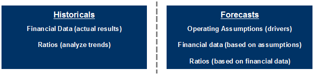
In short, historical financial raw data, and ratios calculated from them, are used as an integral part of the process to derive forward-looking assumptions that drive financial data projections. We should start by building a model designed to reflect that.
Also, as a reminder from the Discounted Cash Flow chapter (as well as the previous chapter), use the mnemonic “C.V.S.” to avoid common errors and help ensure that the outputs of your model will be reasonable:
- Confirm historical financials for accuracy.
- Validate key assumptions for projections.
- Sensitize variables driving projections to build a valuation range.
Model Design & Layouts
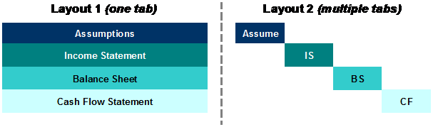
Three-statement financial models can be built in a variety of different layouts and designs. For example, the Income Statement, Balance Sheet, and Statement of Cash Flows can be combined on one excel tab, or each of the three financial statements can occur on separate tabs (i.e., worksheets within a single workbook). The Assumptions can be listed on a separate worksheet, or they can be listed below or beside the Income Statement.
Conceptual vs. Physical Layout
Importantly, however, the analyst must keep in mind the conceptual design of the model. Assumptions are derived from historical financial data as well as logic and external analysis; these assumptions drive the values projected in the Financial Statements (primarily the Income Statement, but as we shall see, the other statements as well). Thus they can be physically on the same worksheet as the statements, but they are always logically separate:
Laying out Assumptions
Likewise, the Assumptions themselves can be built in a variety of layouts. Income Statement drivers and assumptions can be built on a separate tab or as part of the same tab as the Income Statement. If combined on the Income Statement tab, drivers and assumptions can be integrated into the Income Statement or directly underneath the statement line items:
Numeric Display
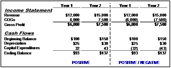
The presentation of the financial statements can be in either a positive-only, or positive/negative, perspective. In other words, numbers that subtract from others (such as Expense items, which subtract from Revenue on the path to calculating Net Income) can be displayed either as positive numbers that are subtracted, or negative numbers that are added. Mathematically, they are equivalent.
Six Steps to Simple Financial Modeling
In Chapter 4, Discounted Cash Flow, we walked you through the basic concepts in projecting Free Cash Flow. In Chapter 7, Financial Modeling, we outlined the key steps in building a complete financial model, and began discussing those steps. Here, we will complete discussing those steps:
- Input historical Financial Statements (Income Statement, Balance Sheet).
- Calculate key ratios on historical financials (e.g., Gross Margin, Net Income Margin, Accounts Receivable/Payable Days, etc.).
- Make forward-looking assumptions for projecting the Income Statement and Balance Sheet based on these historical ratios and any additional considerations.
- Build a Statement of Cash Flows (tying together Net Income from the Income Statement and Cash from the Balance Sheet).
- Tie Ending Cash Balance from the Statement of Cash Flows into the Balance Sheet, and Balance the Balance Sheet.
- Calculate Interest Expense and tie this into the Income Statement.
Because we already went into detail on Steps 1-3 in this process in Chapter 7, we will be expanding on those steps in this chapter. For more detail on Steps 1-3, please revisit that chapter on the Introduction to Financial Modeling.
Step 1: Input Historical Financial Data
The first step in building a financial operating model is to input the historical Financial Statements (Income Statement and Balance Sheet).
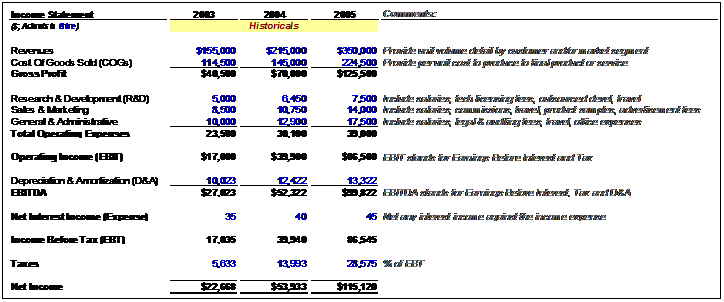
Here are some notes to make this process easier:
- Color code your cells so that formulas are a different color from directly input data. Standard practice is to make the text color blue for input data and black for formulas.
- Put any comments about the line items to the side of each item; standard practice is to make comments italic.
- Use the “Alt + =” shortcut to subtotal the income statement sections. For example, once you input the Operating Expenses items, type “Alt + =” in the cell directly underneath to calculate the subtotal for 2003 of $23,500.
- Double-check that the input data correctly matches the source, and that you end up with the same net income each year as the historical input source. You can code this as a “Balance Check” formula directly in the spreadsheet.
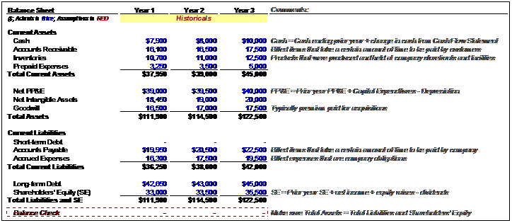
- Follow the same steps for the Balance Sheet by making sure that the input data and formulas match the source. Also, run a “balance check” to make sure the data your input Balance Sheets actually balance. For the Balance Sheet, remember the all-important Accounting Identity:
Total Assets = Total Liabilities + Shareholders’ Equity
Step 2: Calculate Ratios
Once you’ve finished inputting the historical data on the Income Statement and Balance Sheet, you can calculate key historical financial ratios. Make sure to use the relevant ratio when calculating each assumption, which will be used to drive future projections.
Here is a list of ratios typically required, at minimum, to build out Income Statement financial projections:
Year-over-Year Growth Rates: Income Statement
- Revenue: (Year 2 Revenue ÷ Year 1 Revenue) – 1
- Gross Profit: (Year 2 Gross Profit ÷ Year 1 Gross Profit) – 1
- EBIT: (Year 2 EBIT ÷ Year 1 EBIT) – 1
- Net Income: (Year 2 Net Income ÷ Year 1 Net Income) – 1
Margin and Ratio Analysis: Income Statement
- Cost of Goods Sold (COGS): (Year 1 COGS ÷ Year 1 Revenue)
- Gross Margin: (Year 1 Gross Profit ÷ Year 1 Revenue)
- Selling, General & Administrative (SG&A): (Year 1 SG&A ÷ Year 1 Revenue)
- Depreciation & Amortization (D&A): (Year 1 D&A ÷ Year 1 Revenue)
- Effective Tax Rate: (Tax Expense ÷ Earnings Before Tax, a.k.a. EBT)
Compute these for all years in the historical financial data range, noting that growth rate calculations can only begin in Year 2, not Year 1:
Ratio Analysis: Balance Sheet
Next, we must compute ratios on key Balance Sheet line items for each year. Many Balance Sheet ratios are expressed either in terms of units of time (Days), or frequency per unit of time (Turns). Here, we have expressed these ratios as units of time (Days):
- Accounts Receivable Days: 365 days × (Year 1 Accounts Receivable ÷ Year 1 Revenue)
- Inventory Days: 365 days × (Year 1 Inventory ÷ Year 1 COGS)
- Prepaid Expenses: (Year 1 Prepaid Expenses ÷ Year 1 Revenue)
- Accounts Payable Days: 365 days × (Year 1 Accounts Payable ÷ Year 1 COGS)
- Accrued Expenses: (Year 1 Accrued Expenses ÷ Year 1 Revenue)
The use of these historical financial ratios will help you make your assumptions to the financial projections in the future years of the operating model. In this way, you will be able to spot relevant trends in these keys ratios when you project them, and help you reconcile results from the past with the results you are projecting.
Step 3: Assumptions & Forecasts
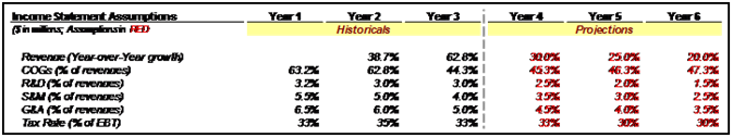
The next step includes building out the projected years (Years 4 to 6) by making assumptions based on the historical data. Typically, you should either use the historical ratios themselves or, where prudent, make assumptions about how these ratios will change over time. To start, let’s look at assumptions for the Income Statement:
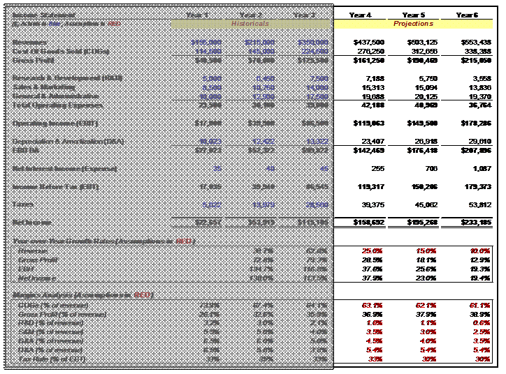
Here are key notes about the assumptions made in red. Please note, for the following discussion, that Sales and Revenue are synonymous:
Year-over-Year Growth Rate Assumptions
- Revenue: The company grew by very high rates in Years 2 and 3. We therefore assume that revenue growth will slow down in upcoming years, but still be strong. The 25%, 15% and 10% are independent variables, or assumptions—they drive the model’s revenue projections, rather than being calculated from revenue. To calculate Year 4 Revenue, we simply take (1 + 25%) × Year 3 Revenue. If this formula is built correctly, we can copy the formula for each year following.
Margin and Ratio Assumptions
- COGS: When a company grows, it is standard to assume that, all other things being equal, Gross Margin will improve (that is, COGS as a percentage of Revenue will decline). The reason for this, as discussed in the previous chapter, is operating leverage. Typically, we assume an incremental improvement each year, such as a 1% decline in COGS as a percentage of Sales. To calculate Year 4 COGS/Sales, we simply take Year 3 COGS/Sales and subtract 1%. Then, Year 4 COGS = (Year 4 COGS/Sales Assumption × Year 4 Sales), where “Year 4 COGS/Sales Assumption” = (Year 3 COGS/Sales) – 1%. We then subtract 1% each year from COGS/Sales in Years 5 and 6 and copy the COGS formula over. In this way, we are modeling a 1% incremental improvement in Gross Margin each year.
- R&D: Again, we can keep R&D/Sales constant, or use an incremental improvement number each year. Here, we have assumed a 0.5% annual reduction in R&D as a percentage of Sales. To calculate Year 4 R&D/Sales, we take Year 3 R&D/Sales and subtract 0.5%. Then, Year 4 R&D Expense = (Year 4 R&D/Sales Assumption × Year 4 Sales), where “Year 4 R&D/Sales Assumption” = (Year 3 R&D/Sales) – 0.5%. We then subtract 0.5% each year from R&D/Sales in Years 5 and 6 and copy the R&D Expenses formula over. In this way, we are modeling a 0.5% incremental reduction in R&D Expenditures as a percentage of Sales in each year.
- SG&A: These forward-looking ratios are modeled exactly the same way. In this model, we have assumed 0.5% annual reductions in both Sales & Marketing (S&M) and General & Administrative (G&A) as a percentage of Sales, thereby reducing total SG&A Expenses as a percentage of Sales by 1% in each year.
- D&A: For Depreciation and Amortization, we make the simplifying assumption that D&A will remain constant as a percentage of Sales. (A more in-depth operating model would forecast Capital Expenditures (CapEx) in each year, and then make assumptions about how much each year’s CapEx would be depreciated in subsequent years.) To calculate this simple version, take the average D&A of Years 1 through 3 (5.4% of Sales) and keep that ratio constant going forward. In modeling D&A this way, we assume that D&A expenses will increase as a constant percentage of Sales, and therefore grow by the same annual percentage that Revenue grows.
- Tax Rate: Typically we estimate historical tax rates and project them as a constant percentage going forward. However, sometimes we can project that tax rates will change, for any of a number of reasons. To illustrate this concept, in this model we’ve kept the Year 3 Tax Rate (as a percentage of Earnings Before Tax, or EBT) of 33% constant in Year 4, but have reduced it to 30% in Years 5 and 6. We might model it this way if we knew that favorable tax treatment was coming a year down the line, perhaps from a business shift to lower-taxation markets, or an anticipated change in statutory tax rates.
Once the key Income Statement assumptions have been made, we can build out the income statement line items as described to compute projected Income Statement results all the way down to Net Income, with one important exception (for now). We leave the “Net Interest Income (Expense)” line item empty, which we will only link into the model as a last step. This is because Net Interest Expense links to the other financial statements, which creates circular calculation dependencies in the model (in a nutshell, circular dependencies occur when A is used to calculate B, which is used to calculate C, which is then used to calculate A). If we make a mistake in this link, it can cause a serious error in the spreadsheet which can become very difficult to fix. Therefore, in the EBT line item, add the Net Interest Income (Expense) line item to the Operating Income (EBIT), but leave the Net Interest Income (Expense) line item completely blank at first. We will link it into the final model later.
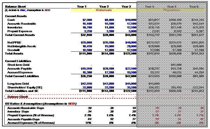
Next, let’s move on to assumptions used to drive projections in the Balance Sheet:
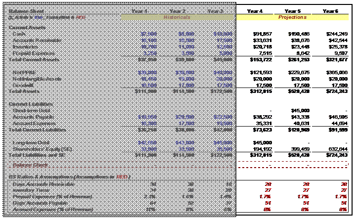
Here are key notes about the assumptions made in red. Because Balance Sheet ratios are typically more difficult to project, we often refrain from changing the assumptions driving these financial results, and instead defer to historical results. Also these assumptions tend to have less of an impact on Valuation results than do Income Statement assumptions. Please note in this discussion that Sales and Revenue are synonymous:
Balance Sheet Ratio Assumptions
- Accounts Receivable Days: Take the average of Accounts Receivable Days from Years 1 through 3, which is 28 days, and keep that number constant in the forecasted years. We can also make assumptions about changes in this ratio if we want, but for the purposes of this model, we have assumed that the ratio stays constant.
- Inventory Days: Take the average of Inventory Days from Years 1 through 3, which is 27 days, and keep that number constant in the forecasted years. (Again, we can add increments or decrements to this number in future years if we feel it is appropriate.)
- Prepaid Expenses: Take the average of Prepaid Expenses/Sales from Years 1 through 3, which is 1.7%, and keep that percentage constant in the forecasted years. (Again, we can add increments or decrements to this number in future years if we feel it is appropriate.)
- Days Accounts Payable: Take the average of Accounts Payable from Years 1 through 3, which is 51 days, and keep that number constant in the forecasted years. (Again, we can add increments or decrements to this number in future years if we feel it is appropriate.)
- Accrued Expenses: Take the average of Accrued Expenses/Sales from Years 1 through 3, which is 8%, and keep that percentage constant in the forecasted years. (Again, we can add increments or decrements to this number in future years if we feel it is appropriate.)
Once we have created the Balance Sheet assumptions, we can fill in the Balance Sheet line items while leaving out the Cash, Net PP&E, Debt and Shareholders’ Equity line items. We will derive those Balance Sheet line items later, from the Statement of Cash Flows.
Use the following formulas to build out the relevant Balance Sheet line items:
- Accounts Receivable: (Year 4 Accounts Receivable Days × Year 4 Sales) ÷ 365 days
- Inventory: (Year 4 Inventory Days × Year 4 COGS) ÷ 365 days
- Prepaid Expenses: (Year 4 Prepaid Expenses/Sales × Year 4 Sales)
- Accounts Payable: (Year 4 Accounts Payable Days × Year 4 COGS) ÷ 365 days
- Accrued Expenses: (Year 4 Accrued Expenses/Sales × Year 4 Sales)
Here are a couple of helpful hints at this stage:
- Keep Goodwill and Intangible Assets line items constant going forward. Unless we are modeling potential changes caused by M&A activity, these line items should not be projected to change.
- Calculate all the assumption values before creating the formulas to calculate each line item in the Financial Statements. Creating the assumption first will allow for easy building of the operating model, and easy checking that the operating model is working correctly.
- Once you are finished, you can check that each line item formula is based off the appropriate assumptions. To check the source of the assumptions used in a formula, highlight the cell containing that formula and press “Ctrl + [”. This will highlight the cells that the formula is dependent upon. For example, put the cursor on the Year 4 Revenue line and press the shortcut. If you have built your formula correctly, Excel will now highlight the Year 3 Revenue cell, as well as the Year 4 Revenue growth assumption cell.
Step 4: Building the Statement of Cash Flows
Once we have the majority of the line items projected out for the Income Statement and Balance Sheet, we are ready to build out the Statement of Cash Flows (SCF). The SCF should look something like this:
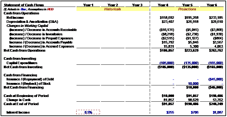
The first line item in the SCF is Net Income from the Income Statement. From this, we take into account all differences between Net Income and the change in the company’s Cash position. There are many—here are the summary points:
- Depreciation and Amortization are generally part of COGS, but they are never actually Cash expenditures—they represent a portion of Capital Expenditures from the past that are being recognized as expenses in the current year. Since they are expenditures in the current year that are not paid for as Cash in the current year, they must be added back to Net Income to account for a company’s change in Cash.
- When the line items of operating assets (things like Accounts Receivable and Inventory) increase, Cash will go down on the SCF. This is because the company has, in effect, spent Cash to build an asset, but hasn’t yet received the Cash back from these assets. For example, from Year 3 to Year 4, the Accounts Receivable line item increases by $16,131; therefore the SCF shows a negative amount of $16,131—the difference between Year 3 Accounts Receivable and Year 4 Accounts Receivable.
- When the line items of operating liabilities (things like Accounts Payable and Accrued Expenses) increase, the opposite happens—Cash will go up on the SCF. This is because the company has, in effect, earned and recorded income from its operations, and thereby accrued liabilities, but hasn’t paid off those liabilities in Cash yet. For example, from Year 3 to Year 4, the Accounts Payable line item increases by $15,792; therefore the SCF shows a positive amount of $15,792—the difference between Year 3 Accounts Payable and Year 4 Accounts Payable.
- Capital Expenditures and Depreciation will dictate the change in Net PP&E. For example, Year 4 Net PP&E = Year 3 Net PP&E + Year 4 Capital Expenditures – Year 4 Depreciation. (Note that in this model, Capital Expenditures have been manually input in the SCF each year, as negative numbers, because they constitute a use of Cash that is not yet reflected in the Income Statement.)
- Net Income and Dividends will dictate the change of Retained Earnings on the Balance Sheet. For example, Year 4 Retained Earnings = Year 3 Retained Earnings + Year 4 Net Income – Year 4 Dividends. (Note that in this model, Shareholders’ Equity is modeled as a single line item in the Balance Sheet – therefore the change in Retained Earnings will be reflected in the change in Shareholder’s Equity.)
- Debt Issuances/(Repayments) can be placed in the cells highlighted in blue based on your assumptions about future changes in debt levels. The same holds for Stock Issuances/(Buybacks). In each case, these Cash inflows/outflows are financing-related, rather than operations-related, and therefore will not be reflected whatsoever in the Net Income calculation. However, they will result in changes to a company’s Cash balance, and therefore must be recorded in the SCF.
- The company’s Change in Cash will equal the sum of the Change in Cash from Operating, Investing and Financing activities. For example, Year 4 Ending Cash Balance = Year 3 Ending Cash Balance + Year 4 Cash from Operations + Year 4 Cash from Investing Activities + Year 4 Cash from Financing Activities.
Step 5: Linking the Three Statements
Now that we have built most of the three financial statements, we can build the final formulas that link, or integrate, all three statements.
- Calculate Net PP&E as Year Prior PP&E + Capital Expenditures (from the SCF) – Depreciation (from the SCF).
- Calculate Long-Term Debt as Year Prior Long-Term Debt + Issuance/(Buyback) of Long-Term Debt (from the SCF). (Note that in this model, a distinction is made between Long-Term Debt and Short-Term Debt, and that the entire Debt balance converts from Long-Term Debt to Short-Term Debt in Year 5 before being repaid in Year 6.)
- Calculate Shareholders’ Equity as Year Prior Shareholders’ Equity + Issuance/(Buyback) of Stock (from the SCF) + Current Year Net Income – Current Year Dividends (from the SCF). (Note that in this model, no Dividends were modeled in the SCF, so the assumed Dividends payment to Shareholders in each year equals $0.)
- Link the Beginning Cash Balance and Ending Cash Balance formulas between the SCF and the Balance Sheet. For example, in Year 4, the Beginning Cash Balance in the SCF should be set equal to the Cash line item for Year 3 on the Balance Sheet. The Cash line item for Year 4 on the Balance Sheet should be set equal to the Year 4 Ending Cash Balance on the SCF. Follow this logic for all years in the financial model. Once you have linked the Cash and remaining line items such as Debt and Shareholders’ Equity, then the Balance Sheet should balance (Total Assets = Total Liabilities + Shareholders’ Equity).
Step 6: Interest Expense (BE CAREFUL!)
At this point the financial model should balance and all balance checks should be affirmed. We have only one piece left to complete: calculating Net Interest Income/(Expense).
As we have discussed before, this calculation flows through all three Financial Statements in the model in what is referred to as a circular calculation (or iterative calculation). When a circular calculation is built, the outputs of a series of calculations become inputs into the same calculation. It is the task of the spreadsheet software to change the values of the different components of the calculation to find a set of values that makes all of the calculations work.
At this stage it is very easy to introduce a mistake into the calculation, and generate an error. Because the calculations are now iterative, any such error will flow through ALL of the calculations, and the entire model will become populated with error messages. (Many an investment banker has gone a sleepless night trying to resolve an accidental error in a circular calculation, so be very careful!)
In order to minimize the chance that you make this mistake, follow these steps exactly:
Avoiding a Circular Calculation Error
- Turn Iterations in the workbook OFF. This can be done through the following Excel menu command: Tools → Options → Calculations.
- Check every formula and make sure the Balance Sheet balances in each projection year.
- Save your workbook. If the following steps introduce an error into your workbook, you should strongly consider closing it without saving it, and re-opening the saved version.
- Calculate Net Interest Income/(Expense) for the first projection year in your model. In the example in this chapter, this would be Year 4. Net Interest Income/(Expense) is calculated as follows:
Interest Income = Assumed Cash Interest Rate × (Prior Year Cash Balance + Current Year Cash Balance) ÷ 2
Interest Income = Assumed Debt Interest Rate × (Prior Year Debt Balance + Current Year Debt Balance) ÷ 2
- If you have built this formula correctly, Excel should complain. It will introduce a dialog box informing you that the calculation is circular. When that box is closed, it will likely open a Help file explaining iterative formulas to you. Close both of these boxes and return to the spreadsheet.
- Turn Iterations in the workbook BACK ON. This can be done through the following Excel menu command: Tools → Options → Calculations.
- If you have computed this correctly, Net Income should have increased/(decreased) by the Net Interest Income/(Expense) amount, and several Balance Sheet items should change slightly (both in the current year and in future years).
- Check every formula and make sure Balance Sheet for the first projection year still balances.
- If everything still looks good, copy the Net Interest Income/(Expense) formula from the first projection year into the remaining, future projection years. Once again, make sure no errors get introduced, and check to make sure the Balance Sheet still balances in all years. (If an error gets introduced, strongly consider closing it without saving it, and trying again with the saved file.)
- If your Balance Sheet still balances and the Interest calculations appear correct, then SUCCESS!
Final Checklist
Congratulations—you are done building your integrated, three-statement financial model! Here are just a few things to consider and check before considering the model 100% complete.
- Never hardcode any number in a formula. Check formula cells to make sure there are no hardcoded values or assumptions in them.
- Make sure that, where applicable, assumptions are the first inputs in each calculation formula.
- Check to see if the trend of each important line item is gradually increasing or decreasing rather than exponentially increasing or decreasing. If you have exponential patterns, you should probably change the assumptions driving them.
- Insert any relevant comments (you can use the shortcut “Shift + F2”) to help other teammates understand your model and assumptions.
- Press “Ctrl + Home” on each worksheet in the Excel workbook so that cursor is on cell A1 in each sheet, before sending the model to your teammates.