In this Financial Modeling chapter we will cover four key topics:

• Financial Modeling Overview
• Model Drivers
• Modeling Revenue Trends
• Modeling Expense Line Items

Financial Modeling Overview

Remember, there are three main Financial Statements commonly used to analyze a company: the Income Statement, the Balance Sheet, and the Statement of Cash Flows. In this module, will dissect financial modeling primarily through the Income Statement. A financial analyst must understand how to evaluate the historical Income Statement line items and make key, rational forward-looking assumptions of the company’s business performance.

Why do we create financial models?

A financial model is built to study a company’s financial history and to use the information available (both past and present) to predict the company’s performance in the future. Although companies change to some degree every year, you can still learn a lot about a company’s revenue growth profile, cost structure, margins, and earnings growth by analyzing its past performance. Likewise, sometimes current information is available that supersedes the past (such as a new acquisition or changed cost structure). These are all essential factors in determining how much a company is worth.

How far out is it reasonable to forecast?

The further out a forecast is made, the less confidence one can have in the accuracy of predictions in it. For this reason, most investment banking models are forecast out only five years, while equity research models are more short-term: they usually only go out two years. Any prediction beyond this horizon is, typically, too uncertain—so many things can change in that timeframe.

What unit of time should be used in the forecast?

Most models are built quarterly or yearly, but in certain circumstances it may make sense to model a business on a monthly basis. For example, if a company is very cash-constrained it may make sense to understand monthly cash flows, as they may not last a quarter. Additionally, some businesses are highly seasonal, and therefore some months of the year look much different from others. In general, you should build your model on an annual or quarterly basis unless instructed otherwise.

What key metrics are predicted?

Generally, a financial model is used to predict several key metrics of a company’s financial performance, with the later items being key metrics in valuing a business:

• Revenue growth
• Gross Profit
• EBIT and EBITDA
• Net Income
• Free Cash Flow

What are the key steps in building a financial model?

In Chapter 4, Discounted Cash Flow, we walked you through the basic concepts in projecting Free Cash Flow. In this module we will take a deeper look at each step in the process—but first, as a review, here are the primary steps involved in building a spreadsheet financial model for a company:

1. Input historical Financial Statements (Income Statement, Balance Sheet).
2. Calculate key ratios on historical financials (e.g., Gross Margin, Net Income Margin, Accounts Receivable/Payable Days, etc.).
3. Make forward-looking assumptions for projecting the Income Statement and Balance Sheet based on these historical ratios and any additional considerations.
4. Build a Statement of Cash Flows (tying together Net Income from the Income Statement and Cash from the Balance Sheet).
5. Tie Ending Cash Balance from the Statement of Cash Flows into the Balance Sheet, and Balance the Balance Sheet.
6. Calculate Interest Expense and tie this into the Income Statement.

It is important to leave the Interest Expense item for last. The main reason for this is that Interest Expense is a function of Debt balances and Cash balances. However, Interest Expense also affects Net Income, which is used to project Cash (and often Debt balances as well). As you can see, there is usually a circular relationship between Interest Expense and Cash/Debt, spanning across the three projected Financial Statements that you’ve built.

Once the circular component of the model has been built, it is very easy to make a mistake that flows through the entire model, and involves a fair amount of work to correct. Therefore, build everything else first, make sure that it is built properly, save the file, and ONLY THEN tie the Interest Expense piece into the model as a final step.

This chapter will discuss the first 3 steps in the above list in detail, while the next chapter, Three-Statement Financial Modeling, will go more in-depth on the technical nitty-gritty to bring your financial model to completion.

Also, as a reminder from the Discounted Cash Flow chapter, use the mnemonic “C.V.S.” to avoid common errors and help ensure that the outputs of your model will be reasonable:

• Confirm historical financials for accuracy.
• Validate key assumptions for projections.
• Sensitize variables driving projections to build a valuation range.

Model Drivers

When building a model, you will generally be faced with a number of considerations about how exactly to build it. One such consideration is how detailed to make the model—should projecting the Income Statement be done in a relatively simple, straightforward way, or should a number of different assumptions (model drivers) be driving it?

The general rule is this: more data inputs do not necessarily mean better data output, but the more thought you have put into your assumptions, the more accurate the model is likely to be. Thus “more drivers” (more assumptions) does not always translate into “better model”, but the modeler should put a fair amount of thought into what parameters drive the results of the business. The most important ones should be broken out as separate assumptions that can be modified.

First, let’s start with the top line of the Income Statement: Revenue. The two main drivers of revenue are Price and Volume.

Price, in turn, is driven by both a company’s pricing strategy and inflationary considerations. Volume drivers include industry growth, product demand, and market share, among potentially others.

So to what level of detail should you dive into this hierarchy of drivers? It depends on the task. In some cases, more detail is better; in others, only a brief overview is required. Usually, models start off relatively simple (a fewer number of drivers) and get more complex as a deal process proceeds (more drivers are added to make the model more sophisticated and more responsive to additional areas of uncertainty).

Continuing with our discussion of revenue drivers, we can look at modeling revenue in one of two primary ways. Revenue can be modeled either top down or bottom up.

Top Down Modeling

Modeling using a top-down approach starts with the addressable market. This is the entire market to which a company could potentially sell its goods or services. The addressable market is then broken down into sub-components.

Most companies will identify the size of their market in their annual 10K filing. You can the calculate the company’s market share by dividing its sales by the total sales for the industry.

Here is an example.

Top-Down Approach To Modeling Unit Sales: Hypothetical Example

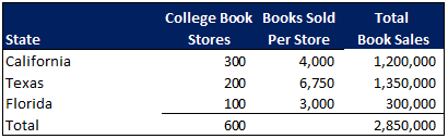
XYZ Corp. operates in California, Texas and Florida and sells college textbooks. Using a top-down approach, we start by studying the percentage of people within each state who attend college:

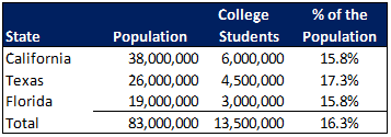
This provides us with the upper bounds of our addressable market. If XYZ Corp only sells to college students in these states, we know they cannot sell books to more than 13.5 million potential customers.

Next, we need to understand XYZ’s market share and how many books each student buys:

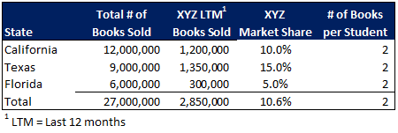
Out of a population of 83 million people, we compute that 13.5 million are college students. If we assume that each college student buys an average of two books per year, there are 27 million (13.5 million × 2 books per student) college textbooks sold annually in these states. Of that, we compute that XYZ Corp has approximately 11% market share (XYZ Books Sold of 2.85 million ÷ Total of Books Sold of 27 million). Note that this share is different in different states—this may become important, especially if we find that expected growth rates differ by state. We estimate this in the next step.

Once we understand the addressable market, we can now forecast the growth rate of the population, the percentage of people that are in college, the total number of textbooks each person in college buys, and the market share XYZ Corp has:

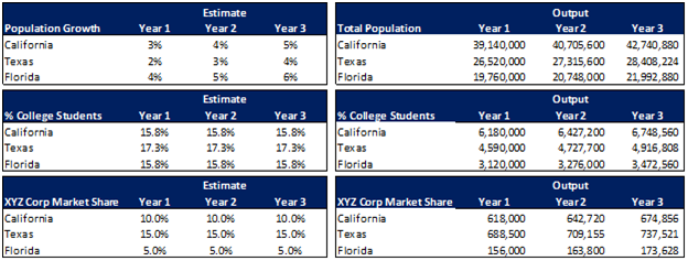
Assumptions:

1. California’s population grows by 3%, 4% and 5% over the next 3 years.
2. Texas’s population grows by 2%, 3%, and 4%.
3. Florida’s population grows by 4%, 5%, and 6%.
4. The percentage of college students in each state stays the same as the previous year.
5. XYZ maintains the same market share each year in each state.

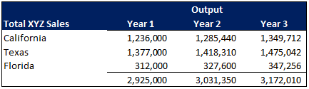
If we estimate that each person continues to buy two books per year, then we project that XYZ Corp will sell almost 3 million books next year, and more than that in Years 2 and 3:

Math Example: In Year 1, California grows population 3%, to 39.1 million × 15.8% college students × XYZ market share of 10% = 618,000 college students. These college students each buy two books per year, so 2 books × 618,000 = 1,236,000 books sold in California in Year 1.

Conclusion: In this example, volume growth was mainly a function of population growth within XYZ Corp’s markets. In order to project revenue, we would then need to make assumptions about projected per-book price increases (or decreases) in each year.

Bottom-Up Modeling

By contrast, modeling using a bottom-up approach is based on the unit economic approach of a single customer or selling unit, regardless of the segmentation. Bottom-up analyses generally rely heavily on historical data from actual sales in the past, and go from there.

Because bottom-up analyses build directly from recent historical results, a bottom-up analysis is typically more accurate in the short-term, and is therefore generally used when estimating short-term trends.

Bottom-Up Approach To Modeling Unit Sales: Hypothetical Example

XYZ Corp sells books to college students, mainly through college bookstores. Thus in our bottom-up approach, unit growth will be mainly a function of store growth and books sold per store:

This analysis disregards the big picture view of population growth, but it does focus on the unit economics of the business, which can be just as accurate (and sometimes, in the short-term, it can be even more accurate).

Now, we need to make assumptions about how this existing market will grow. When forecasting, there are two ways to determine what growth rate to use: historical data and research-based assumptions.

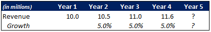
Using historical data is as simple as looking at the historical growth rates, identifying a pattern, and then applying a reasonable assumption for future periods based on this pattern. If XYZ Corp has consistently grown revenues by 5% every year, it seems reasonable to assume that revenue would continue to grow at a similar pace:

It should be noted that this same logic would apply when modeling segments of the addressable market in the top-down approach.

In order to increase the level of accuracy of your estimate, you should also conduct research. Research can involve reading the company’s historical filings to look for clues of what management thinks growth could be. You can also study macro factors or sector-specific factors that may influence the company’s revenue growth rate. For example, since XYZ Corp sells books to college students, college enrollment patterns will likely influence total number of college textbooks sold. Additionally, if XYZ is expanding to new college bookstores, it would be reasonable to make assumptions about how many new stores the company will sell to, and how quickly book sales will accumulate in these new stores.

Conclusion: In this example, volume growth was mainly a function of the number of college bookstores that XYZ Corp sells through. We had the option to grow volume based upon the number of bookstores that the company sells through, and assumptions about growth in book sales per store. We also had the option of modeling new store growth and making assumptions about how many sales these stores will garner for the company. In order to project revenue, we would then need to make assumptions about projected per-book price increases (or decreases) in each year. Instead, we made the simplifying assumption that revenue growth continues at a 5% rate, similar to the company’s recent past revenue growth rate.

Modeling Revenue Trends

Generally speaking, established companies tend to grow revenues over time at an approximate rate—one that can be difficult to measure precisely, but often a range can often be found. However, this long-term underlying growth trend can be obscured by short-term developments caused by specific patterns.

There are three main types of revenue patterns, or trends, to look for: seasonal, cyclical, and secular. When modeling business performance, it is critical to make sure that your assumptions coincide with the economic reality of the company you are modeling.

Seasonal Trends

A seasonal business is one with revenue patterns that increase and decrease with a regular pattern during specific periods of the year. The pattern does not have to be based around seasons, but oftentimes it is (such as housing or road construction in the Northern US).

Here are some concrete examples:

• A company that sells snowplows is likely to do a lot of business in the winter and late fall, but little business in the summer. In this case, the strong sales period lasts about 3-6 months.
• A flower shop will likely see a huge increase in sales in the days leading up to Valentine’s Day and Mother’s Day. These two holidays may represent 75% of the company’s full-year business, with the strong sales period only lasting a couple of days.
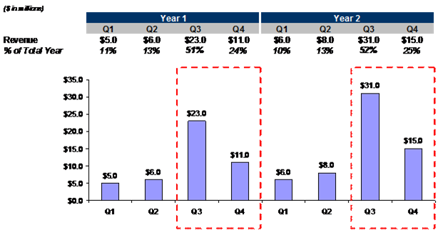
• Retail companies tend to have strong sales performance around the end of the year, with people buying gifts for holidays such as Christmas and Hanukkah.  As you can see in the graphic below, a majority of each year’s revenue occurs in the 3rd and 4th quarters.

Cyclical Trends

A cyclical business is similar to a seasonal business, in that business tends to be strong in certain periods but weaker in others. For cyclical businesses, however, the trend usually lasts for a time period longer than one year (sometimes as long as a decade), and is generally unrelated to the calendar.

Cyclical companies often have long periods of sustained growth followed by a sharp drop off when the cycle changes. What causes this cycle? It depends, but usually the cycle is tied to the strength of some economic indicator, such as gold prices, GDP growth, or new housing starts. For example, the housing market had a long growth period through the early and mid 2000’s, and collapsed in 2007 and 2008. Oil refining business revenues and earnings are closely tied to the price per barrel of oil. Retail companies experience cyclical growth trends around overall GDP growth and/or consumer spending growth.

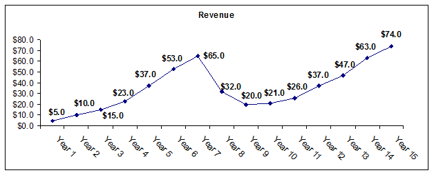
As you can see in the graphic below, the hypothetical company experienced a major decline in its revenue path in Years 8 and 9. This could be due to internal problems specific to the company (such as a major lawsuit or a product safety scare), or due to macroeconomic effects such as a credit crisis or a global growth slowdown. (Depending on the situation, it is also possible that revenue growth in Years 3-7 was exaggerated due to the same cyclical indicator that lead to the downturn in Years 8-9.)

Secular Trends

A secular trend typically lasts longer than a cyclical trend. It typically involves the advent of a new technology or consumer behavior that is here for good, or at least for a long time. The reserve is also true: some business are involved in secular declines due to technological obsolescence, or shifts away from them in consumer behavior.

For example, the Internet is a new technology that has revolutionized many industries, and has been consistently growing for the past 20 years and will likely continue to for some time. By contrast, outdated technologies such as CDs and DVDs are in decline after being replaced by online media and Blu-Ray technology. Another industry in secular decline is milk production, as adults shift to other sources of calcium and protein, partly due to available substitutes and partly due to health concerns.

In the graphic below, the blue line represents the revenue of a company that is experiencing secular growth while the pink line represents a company that operates in a secular decline.

Modeling Expense Line Items

The cost structure of a business’s operations can be divided into two components: fixed costs and variable costs. Fixed costs tend not to change as a company’s revenue grows or declines, while variable costs are directly related to how much revenue a company is earning.

Costs can also be divided into production-related expenses (often called Cost of Goods Sold, or COGS), and non-production-related expenses (often called Other Operating Expenses or just Operating Expenses).

Fixed Costs

Fixed costs typically stay constant year over year, unless the company puts a cost savings program into place, such as by firing corporate headquarters employees. Examples of fixed costs are rent payments, management salaries, and insurance premiums.

Variable Costs

Variable costs are usually directly related to the production and supply of goods or services available for sale, and are typically modeled as a percentage of revenue. Examples include labor, material, and utility costs.

As a company grows revenue and keeps fixed costs in place, a company is able to increase its profitability. This arises from a phenomenon known as operating leverage. Operating leverage measures the degree to which profit as a percentage of revenue grows as revenue grows. Companies with a high fixed cost structure tend to exhibit the most operating leverage.

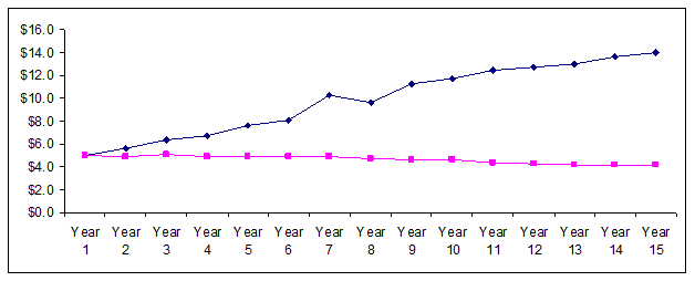
Here’s an example: a company may be utilizing half of its current manufacturing facility. As new orders come in for its products, the company is able to produce more products without utilizing an additional facility. Thus, the percentage of revenue that can be saved as gross profit increases as the number of units produced increases. As you can see in the graphic below, the hypothetical company has increased its revenue and its gross margin simultaneously.

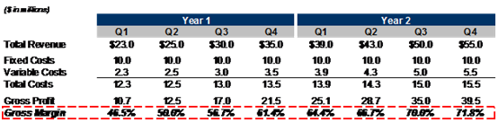
It is important to note that Variable Costs are not synonymous with COGS, and likewise, Fixed Costs are not synonymous with Other Operating Expenses. True, many COGS expenditures tend to be variable—but not all of them are. Likewise, some non-production-related Operating Expenses, such as Sales & Marketing, tend to vary proportionally with revenue.

SG&A: Head Count, Marketing, and Corporate Expenses

Selling, general and administrative expenses are typically modeled as a percentage of revenue. Investment bankers typically evaluate the SG&A as a percentage of revenue over the last few historical years and make assumptions (e.g., by taking the average of the last three years). It is important to note, however, that typically, at least some component of SG&A is actually fixed expenses. Costs like insurance premiums, legal counsel, and corporate employee salaries tend to be mostly fixed, at least in the short-term.

EBIT and EBITDA

After COGS and Other Operating Expenses are subtracted out, the result is EBIT. EBIT is short for Earnings Before Interest and Taxes, and EBITDA is EBIT plus Depreciation and Amortization Expenses. EBIT is also called Operating Profit, because it is the money produced by the operations of the company before Taxes and Interest are taken out. EBITDA takes this one step further by removing the non-cash expenses, Depreciation and Amortization. EBITDA is a proxy for the cash flow of the operations of a business, assuming that no new Capital Expenditures are necessary. This is usually not the case, however, because ongoing operations usually need more capital expenditure to grow the company and to maintain the business infrastructure in place.

It is important to understand that EBITDA and EBIT are not drivers of a financial model. They are among the primary outputs of the model. They are key metrics that investment bankers use to evaluate the worth of a business.

Modeling Interest Expense and Interest Income

Interest Expense and Income are based directly off the outstanding Debt and Cash balances, respectively, that a company shows on its Balance Sheet. To model these on a going forward basis:

• Divide Interest Expense by total Debt amount to calculated the average Cost of Debt (prior to any adjustments for the Tax Shield of Debt—more on this in later chapters and in Chapter 4, Discounted Cash Flow).
• Check to see if the company has any swaps outstanding, or anything else that may change the implied average Cost of Debt.
• Model future Interest Expense as the average Cost of Debt multiplied by the average amount of Debt on the Balance Sheet in each year. This is usually calculated as: (Beginning Debt Balance + Ending Debt Balance) ÷ 2.
• For Interest Income, try to determine how much of the Cash balances have historically been invested in interest-bearing assets; use previous Interest Income figures to determine the average interest rate earned on these balances. Then, make assumptions about this rate in the future, and multiply this assumed rate by the average amount of Cash on the Balance Sheet in each year. As with Debt, this is usually calculated as: (Beginning Cash Balance + Ending Cash Balance) ÷ 2.

Taxes

Once Net Interest Expense has been computed, subtract it from EBIT to arrive at EBT (Earnings before Tax). In order to estimate future tax rates on EBT, look at historical effective tax rates (different from marginal tax rates, in that effective tax rates measure the total percent of EBT that is paid as taxes, while marginal tax rates measure the amount of tax liability generated from a $1 additional increase in EBT).

In addition, read annual and quarterly filings to see if there are any reasons why effective taxes may be higher or lower than historical rates (e.g., because of R&D tax credits, Net Operating Losses (NOLs), changes in statutory corporate tax rates, or changes in exposure to foreign countries). Take out one-time expenses or non-recurring items that may have impacted the tax rate in previous years. If the company has a NOL carryforward, which may act as a tax shield protecting future profits from taxation, use a normalized tax rate in projecting future tax rates. The NOL carryforward can be valued separately as a tax shield, assuming that the company remains profitable in the future.

Net Income

Once taxes have been subtracted from EBT, we have Earnings, or Net Income. Like EBIT and EBITDA, Net Income can be used in some models as a basis for valuation – particularly if we are valuing the equity component of a business (Market Capitalization) separately from the business as a whole (Enterprise Value).

Calculate Earnings Per Share

Net, we can estimate Earnings Per Share (EPS). EPS is simply the ratio of Net Income to Number of Outstanding Shares. EPS comes in two varieties: Basic EPS and Fully Diluted EPS.

• Basic EPS: Net Income ÷ Weighted-Average Shares Outstanding—(Beginning SO + Ending SO) ÷ 2.
• Fully Diluted EPS: Net Income ÷ Average Fully-Diluted Shares Outstanding—(Beginning FDSO + Ending FDSO) ÷ 2.

In the Fully-Diluted Shares Outstanding calculation, be sure to include all options, warrants,  convertible bonds, and convertible preferred shares as though they were converted today into outstanding shares. This makes the denominator of the EPS calculation as large as it can reasonably be, and is thus an ultra-conservative measure of a firm’s earning power.

You may need to adjust your outstanding share assumptions if new equity shares are being issued or if shares are being repurchased through a share buyback plan. If a share buyback plan is operational, read the financial statements and company filings to try to understand how many more shares are remaining to be repurchased on the existing share buyback authorization. Assume that the company will use a certain percentage of cash flow to buy back stock, and model out the future outstanding share amounts using this assumption.

Other Notes

• Calculate Debt/EBITDA: The Debt/EBITDA ratio is a measure of the financial leverage of a company. This metric is an indicator of how much wiggle-room the company has to pursue different corporate actions, including share buybacks. When doing share buyback modeling, understand how much leverage the company can reasonably take on if you are assuming that the company is using cash flow to buy back stock rather than pay down debt.
• Calculate EBITDA/Interest Expense: The EBITDA/Interest Expense ratio is a measure of a company’s ability to service its debt—i.e., how much of the cash flow from its operations is being used to compensate the holders of the company’s debt. If this ratio begins approaching 1 (or worse, is at or below 1!), then the company is spending most or nearly all of its EBITDA to pay for its existing Debt—a potentially dangerous sign. Likewise, if EBITDA is declining, watch this metric to understand if company will have any issues servicing its existing Debt obligations.

←Initial Public OfferingsThree Statement Financial Modeling→