When interviewing for a junior private equity position, a candidate must prepare for in-office modeling tests on potential private equity investment opportunities—especially LBO scenarios. In this module, we will walk through an example of an in-office LBO modeling test. In-office case studies and modeling tests can occur at various stages of an interview process, and additional interviews with other members of the private equity team could occur on the same day. Therefore, you should strive to be able to do these studies effectively and efficiently without draining yourself so much that you can’t quickly rebound and move on to the next interview. Make sure to take your time and build every formula correctly, since this process is not a race. There are many complex formulas in this test, so make sure you understand every calculation.
This type of LBO test will not be mastered in a day or even a week. You must therefore begin practicing this technique in advance of meeting with headhunters. Repeated practice, checking for errors and difficulties and learning how to correct them, all the while enhancing your understanding of how an LBO works, is the key to success.
- Investment Scenario Overview
- Given Information (Parameters and Assumptions)
- Exercises
- Step 1: Income Statement Projections
- Step 2: Transaction Summary
- Step 3: Pro Forma Balance Sheet
- Step 4: Full Income Statement Projections
- Step 5: Balance Sheet Projections
- Step 6: Cash Flow Statement Projections
- Step 7: Depreciation Schedule
- Step 8: Debt Schedule
- Step 9: Returns Calculations
Given Information (Parameters and Assumptions)
Below we provide the given information from a real-life LBO test that was given to a pre-MBA associate candidate at a large PE firm. We will use it as an example of how to build an LBO model from scratch during the interview. Remember that candidates will receive a laptop and a printout with key information regarding the transaction to complete this assignment.
ABC Company, Inc.
Scenario Overview and Revenue Assumptions:
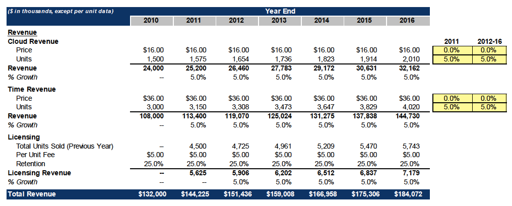
ABC Company, Inc. is a developer of software applications for smartphone devices. The company sells two products for the various smartphones. The first is a software application called Cloud that tracks weather data. The second application, Time, acts as a calendar that keeps track of a user’s schedule. ABC Company prices Cloud at $16.00 and Time at $36.00 per software license. ABC Company sold 1.5 million copies of Cloud and 3 million copies of Time in 2010. That was the first year ABC Company generated any revenue.
Each software application requires the payment of a $5.00 renewal fee every year. ABC Company renews approximately 25% of the licenses it sold in the prior year; this renewal fee acts as a source of recurring revenue. To simplify, assume that renewals happen for only one additional year and that the recurring revenue stream is based on the prior year’s new licenses. Note that ABC Company does not incur any additional costs for renewals.
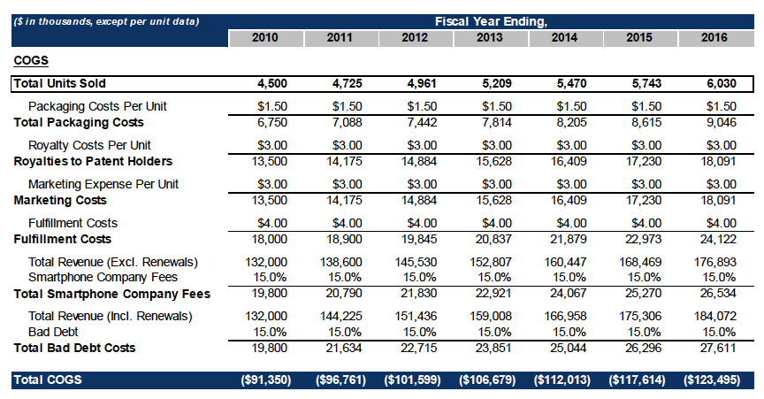
COGS assumptions (assume constant throughout the projection period):
- Packaging costs = $1.50 per unit
- Royalties to technology patent owners = $3.00 per unit
- Marketing expense = $3.00 per unit
- Fulfillment expense = $4.00 per unit
- Fees to smartphone companies = 15% of sale price (does not include renewal fees)
- ABC Company incurs a 15% bad debt allowance on total revenues (consider this as part of cost of sales, wherein ABC Company is unable to collect from customers’ credit card companies).
G&A and other assumptions (assume constant throughout the projection period):
- Rent of development property and warehouse facilities = $350,000 annually
- License fee to telecom internet providers = $1.5 million annually
- Salaries and benefits = $1.75 million annually
- Sales commissions = 5% of all sales including renewals
- Offices and other administrative costs = $750,000 annually
- CEO salary and bonus = $1.25 million annually + 3% of all sales including renewals
- Federal tax rate = 35% and state tax rate = 5% on EBT
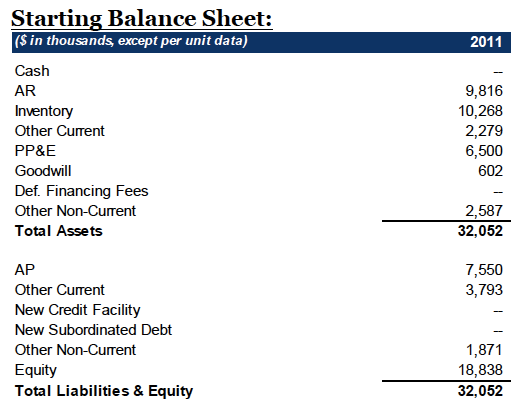
Starting Balance Sheet:
Investment Assumptions:
Due to the depressed macroeconomic and investing environment, the PE fund is able to acquire ABC Company for the inexpensive purchase price of 5.0x 2011 EBITDA (assuming a cash-free debt-free deal), which will be paid in cash. The transaction is expected to close at the end of 2011.
- Senior Revolving Credit Facility: 3.0x (2.0x funded at close) 2011 EBITDA, LIBOR + 400bps, 2017 maturity, commitment fee of 0.50% for any available revolver capacity. RCF is available to help fund operating cash requirements of the business (only as needed).
- Subordinated Debt: 1.5x 2011 EBITDA, 12% annual interest (8% cash, 4% PIK interest), 2017 maturity, $1 million required amortization per year. (Hint: add the PIK interest once you have a fully functioning model that balances.)
- Assume that existing management expects to roll-over 50% of its pre-tax exit proceeds from the transaction. Existing management’s ownership pre-LBO is 10%.
- Assume a minimum cash balance (Day 1 Cash) of $5 million (this needs to be funded by the financial sponsor as the transaction is a cash-free / debt-free deal).
- Assume that all remaining funding comes from the financial sponsor.
- Assume that all cash beyond the minimum cash balance of $5 million and the required amortization of each tranche is swept by creditors in order of priority (i.e. 100% cash flow sweep).
- Assume that LIBOR for 2012 is 3.00% and is expected to increase by 25bps each year.
- The M&A fee for the transaction is $1.5 million. Assume that the M&A fee cannot be expensed (amortized) by ABC and will be paid out of the sponsor equity contribution upon close.
- In addition, there is a financing syndication fee of 1% on all debt instruments used. This fee will be amortized on a five-year, straight-line schedule.
- Assume New Goodwill equals Purchase Equity Value less Book Value of Equity.
- Assume Interest Income on average cash balances is 1%.
Hint: The first forecast year for the model will be 2012. However, you will need to build out the income statement for 2010 and 2011 to forecast the financial statements for years 2012 through 2016.
Exercises:
- Build an integrated three-statement LBO model including all necessary schedules (see below).
- Build a Sources and Uses table.
- Make adjustments to the closing balance sheet of ABC Company post-acquisition.
- Build an annual operating forecast for ABC Company with the following scenarios (using 2010 as the first year for the revenue forecast; note that 2010 EBITDA should be approximately $25 million). Assume that in 2011 there is 5% growth in units sold (both Cloud and Time units).
- 2012-2016 assumptions include:
- Upside Case: 5% annual growth in units sold (both Cloud and Time units)
- Conservative Case: 0% annual growth in units sold (both Cloud and Time units)
- Downside Case: 5% annual decline in units sold (both Cloud and Time units)
- Build a Working Capital schedule using Accounts Receivable Days, Accounts Payable Days, Inventory Days, and other assets and liabilities as a percentage of Revenue. Assume working capital metrics stay constant throughout the projection period and assume 365 days per year.
- Build a Depreciation Schedule that assumes that existing PP&E depreciates by $1 million per year, and that new capital expenditures of $1.5 million per year depreciate on a five-year, straight-line basis.
- Build a Debt schedule showing the capital structure described earlier. Use average balances for calculating Interest Expense (except for PIK interest—assume that PIK interest is calculated based on the beginning year Subordinated Debt balance and not the average over the year).
- Create an Exit Returns schedule (including both cash-on-cash and IRR) showing the returns to the PE firm equity based on all possible year-end exit points from 2012 to 2016, with exit EBITDA multiples ranging from 4.0x to 7.0x.
- Display the results of all of these calculations using the “Upside Case.”
Note that the above description incorporates all of the information, assumptions and assignments that were given in this LBO in-person test example.
Step 1: Income Statement Projections
As part of the first step, build out the core operating Income Statement line items for years 2010 through 2016.
- Make a distinction between 2011 assumptions and 2012-2016 assumptions
- Take the provided assumptions and make the revenue and cost build based upon them.
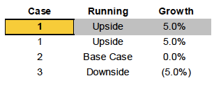
- OFFSET is a simple Excel formula that is used commonly to interchange scenarios, especially if the model becomes very complex. It simply reads the value in a cell that is located an appropriate number of rows/columns away, based on the parameters given to the function. Thus, for example, =OFFSET(A1, 3, 1) will read the value in cell B4 (3 rows and 1 column after A1).
Next, build the costs related to Revenue based upon the information given in the case.
Then, build the G&A expenses from the given information.
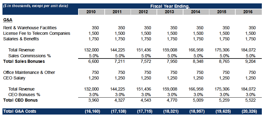
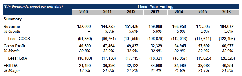
Finally, build a simple summary schedule for the above projections.
Step 2: Transaction Summary
As part of the second step, build out the transaction summary section which will consist of the Purchase Price Calculation, Sources and Uses, and the Goodwill calculation.
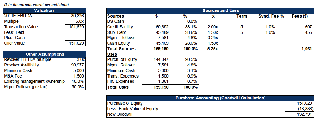
- This model assumes a debt-free/cash-free balance sheet pre-transaction for simplification. Without debt or cash, the transaction value is simply equal to the offer price for the equity (before fees and minimum cash—discussed below).
- The funding for this model is fairly simple: the funded credit facility is 2.0x 2011E EBITDA, the subordinated debt is 1.5x, and the remaining portion is the equity funding, which is a combination of management rollover equity and sponsor (PE firm) equity. (Note that the 5.0x 2011E EBITDA is the offer value for the equity before the M&A and financing fees and the minimum cash balance, not after. After fees/cash, it ends up being 5.25x.)
- The management rollover is simply half of the management team’s proceeds from selling the company. Since management owned 10% of the company before the transaction, it constitutes 5% of the offer price for the original equity.
- The sponsor equity is the “plug” in this calculation. In other words, it is the amount that is solved for once all other amounts are known (offer price + minimum cash + fees – debt instruments – management rollover equity).
- The total equity (including management rollover) represents about 30-35% of the funding for the deal, which is about right for a typical LBO transaction.
- Goodwill is simply the excess paid for the original equity (offer price – book value of equity).
Step 3: Pro Forma Balance Sheet
As a next step, build out the Pro Forma Balance Sheet using the given 2011 balance sheet. To do this, you need to incorporate all the transaction and financing-related adjustments needed to produce the Pro Forma Balance Sheet. Each adjustment is discussed in detail below.
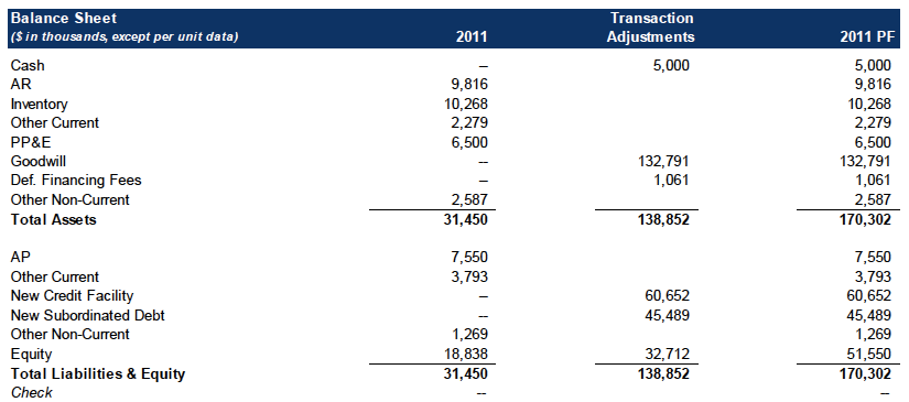
- Since this is a cash-free and debt-free deal to start, there are no Pro Forma adjustments for the cancelling or refinancing of debt.
- Cash increases by $5 million upon close because the sponsor is funding the minimum cash balance (minimum cash that is assumed to be needed to run the business).
- The New Goodwill is simply the purchase value of the equity (not including fees) less the original book value of the equity.
- The adjustment for Debt Financing Fees reflects the cost of issuing the new debt instruments to buy the company. This fee is considered an asset, and is capitalized and amortized over 5 years.
- The Debt-related adjustments reflect the new debt instruments for the new capital structure.
- The Equity adjustment reflects the fact that the original equity is effectively wiped out in the transaction—the “adjustment” amount shown here is simply the difference between the new equity value and the old one. The new equity value will equal the amount of the total equity funding for the transaction (sponsor plus management’s rollover) less the M&A fee, which is accounted for as an off balance-sheet cost.
- VERY IMPORTANT: This stage of the LBO model development (once Pro Forma adjustments have been made to reflect the impact of the transaction on the balance sheet) is a very good time to check to make sure that everything in the model so far balances and reflects the given assumptions. This includes old and new assets equaling old and new liabilities plus equity; new sources of capital equaling the transaction value, which equals the offer price for the original equity (adjusting for cash, old debt and fees), etc.
Step 4: Full Income Statement
Next, build the full Income Statement projections all the way down to Net Income. Note that a few line items (especially Interest Expense!) will be calculated in later steps. Once the Cash Flow section and other schedules are built, link all the final line items to complete the integrated financials.
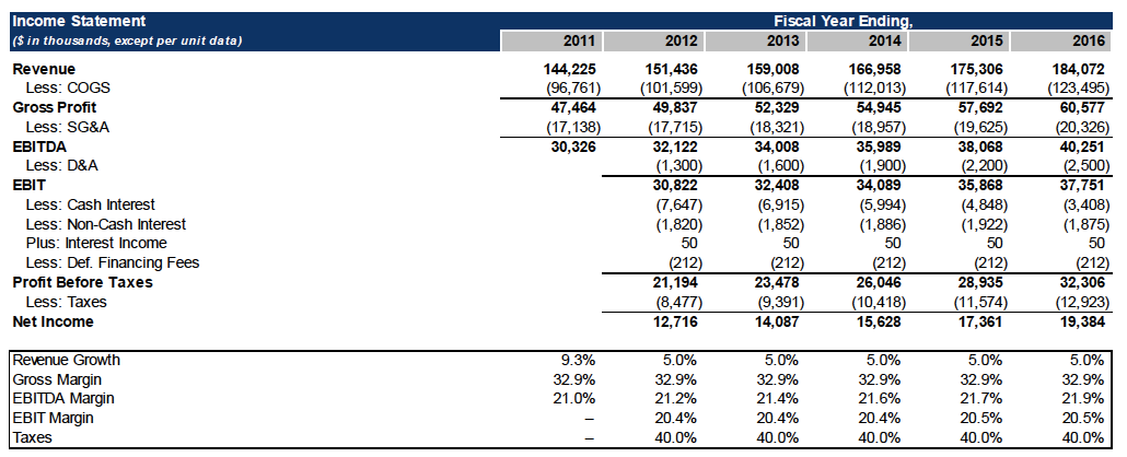
- You can link the Revenue, COGS and SG&A calculations to the operating model (built in Step 1) to get to EBITDA.
- To get from EBITDA to Net Income, set up the framework first (include line items to subtract D&A, and to subtract Interest and fees, to get to EBT. Then subtract taxes to get Net Income—but keep in mind for now that calculating D&A and Interest will come a bit later, from other schedules you have not yet created).
- D&A will be linked to the Depreciation Schedule that you will need to build (schedule of the Depreciation of the existing PP&E and new Capital Expenditures made over the projection period).
- Interest Expense and Interest Income will be linked to the Debt Schedule that you will need to build. There will be a natural circular reference because of the cash flow sweep feature of the LBO model, combined with the fact that Interest Expense is dependent upon Cash balances. This is usually one of the last things you should build in an LBO model.
- The amortization of Deferred Financing Fees is fairly straightforward: it uses a straight-line, 5 year amortization of the fees described in the case write-up and computed in Step 2.
- The tax rates apply to EBT after all of these expenses have been subtracted out. They are given in the case write-up.
Step 5: Balance Sheet Projections
Next, forecast the Balance Sheet from 2011 to 2016. Note that we start with the 2011 Pro Forma Balance Sheet from Step 3, not the original Balance Sheet.
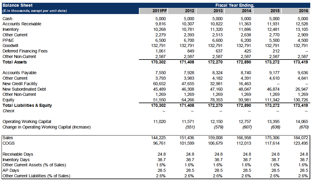
- Laying out the Balance Sheet is similar to laying out the Income Statement—you’ll have to set up the framework for some line items and leave the formulas blank at first, as they will be calculated in the other schedules you will create.
- Cash remains at $5 million throughout the life of the model, as we’re assuming a 100% cash flow sweep and that the minimum cash balance is $5 million. (Cash would only start to increase if we project out long enough that all outstanding Debt is paid off.)
- You’ll need to build out the Operating Working Capital line items (Accounts Receivable, Inventory, Other Current Assets, Accounts Payable, Other Current Liabilities) according to the assumptions stated in the case write-up.
- Accounts Receivable (AR): Calculate AR days (AR ÷ Total Revenue × 365) for 2011 and keep it constant throughout the projection period.
- Inventory: Calculate Inventory days (Inventory ÷ COGS × 365) for 2011 and keep it constant throughout the projection period.
- Other Current Assets: Keep this line item as a constant percentage of revenue throughout the projection period.
- Accounts Payable (AP): Calculate AP days (AP ÷ COGS × 365) for 2011 and keep it constant throughout the projection period.
- Other Current Liabilities: Keep this line item as a constant percentage of revenue throughout the projection period.
- Total Deferred Financing Fees are computed based upon the Debt balances and percentage assumptions given in the model. Deferred financing fees are then amortized, straight-line, over 5 years.
- The Credit Facility and Subordinated Debt line items will link to your Debt schedule. Their balances will decrease over time as a function of the cash available for Debt paydown (since the case write-up specifies a 100% cash sweep function).
- Equity (specifically Retained Earnings) will increase each year by the same amount as Net Income, because there are no dividends being declared. If dividends were to be added into the model, you would calculate ending Retained Earnings as Beginning Retained Earnings + Net Income – Dividends Declared.
- As discussed earlier, the balance sheet has the pleasing feature that if it balances, the model is probably operating correctly! Now is another good time to make sure everything balances before proceeding.
Step 6: Cash Flow Statement Projections
Next, forecast the Cash Flow Statement as requested in the Exercises section.
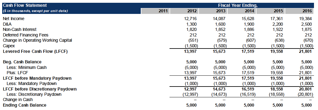
- Start with Net Income and add back non-cash expenses from the Income Statement, such as D&A, Non-Cash Interest (PIK), and Deferred Financing Fees.
- Next, subtract uses of Cash that are not reflected in the Income Statement. These include the increase in Operating Working Capital (which you calculated using your balance sheet) and Capital Expenditures (which is calculated here or, alternatively, could be calculated in the Depreciation Schedule to be built shortly).
- Next, calculate the change in cash, which will be interconnected with the Debt schedule. In this case, the model is assuming a 100% cash flow sweep (after mandatory debt amortization payments), so cash should not change after the 2011PF Balance Sheet amount of $5 million.
- Even though the amount is not changing, the Cash line item should link back to the Balance Sheet. This is because the model could later be used to relax the assumption that 100% of excess cash is swept to pay down Debt. If it’s less than 100%, Cash would accumulate, and that would need to tie in to the other financial statements.
Step 7: Depreciation Schedule
Next, forecast the Depreciation schedule as requested in the Exercises section.
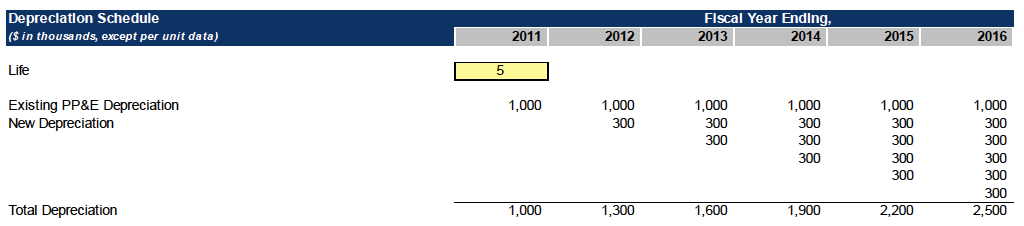
- The original PP&E is depreciated $1 million annually, as stated in the assumptions.
- New Depreciation is calculated based on the annual investment in Capital Expenditures over the projection period. This new Depreciation is created using a waterfall (see above): each year new Capital Expenditures occur and need to be depreciated; each year, Capital Expenditures from previous projection years in the model may have to be partially depreciated in that year. The sum of all of the component Depreciation line items (one row for each year, plus the Depreciation on the original PP&E) gives the total Depreciation Expense for the year.
Note that this model is less complex than it could be. Given that Capital Expenditures do not change each year, and that each new Capital Expenditure is depreciated according to the same simple schedule, the numbers and calculations are fairly straightforward. Here, we’re simply assuming that new Capital Expenditures are expensed evenly over a 5 year period (using straight-line depreciation), as specified in the case write-up.
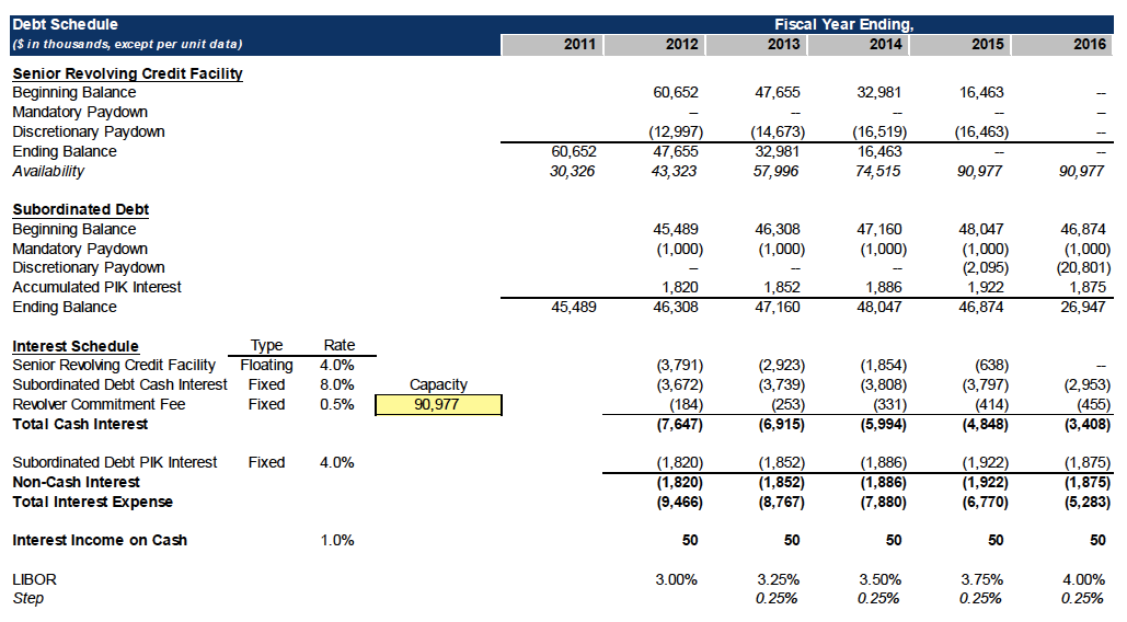
Step 8: Debt Schedule
Next, forecast the Debt Paydown and Interest Expenses for each year via the Debt Schedule, as requested in the Exercises section.
- We need to build this schedule correctly! The Debt Schedule is probably the trickiest part of the LBO model to build—especially for anyone who has not built an LBO model before. The Debt Schedule will create the circular (iterative) reference that is the defining characteristic of a true LBO model. Before linking the Debt, Cash, and Interest calculations to one another in the Debt schedule, be sure to turn “Iterations” on in the Formulas section of Microsoft Excel’s Options menu.
- WARNING: Be very careful about changing formulas once you have built the iterative calculation. If you do so and introduce an error, it could bust your entire model if you’re not careful. This is because the error will travel all the way through the iterative calculations and end up everywhere! If you run into this problem, break the circular reference entirely (by deleting it), reconstruct the calculations for the first forecast year (2012), and then copy and paste them across the columns, one year at a time (2013, then 2014, etc.). Many PE professionals have spent late nights in the office trying to recover from an accidental error introduced into a circular LBO model formula!
- To compute the changes in Debt balances, calculate LFCF (the framework for this started already on the Statement of Cash Flows). This determines how much debt is going to be paid down (both discretionary and non-discretionary).
- The non-discretionary portion is the required amortization payments made on debt (in this case, there is only required pay-down for subordinated debt).
- The discretionary portion is the sweep portion of the remaining LFCF less required amortization. Since we’re assuming a 100% cash flow sweep, all of the LFCF is used to pay down debt—first the Senior Credit Facility, then the Subordinated Debt. The cash flow sweep and required payments will help you calculate the beginning and ending balances of both of the debt tranches.
- The Senior/Revolving Credit Facility (S/RCF) is the first priority to get paid off via the cash flow sweep. It should be completely paid off before later tranches receive any discretionary principal repayment in the Debt Schedule.
- Also note that we need to include a fee for the availability of the unused portion of the RCF, even if the business never uses it—this is a typical, annual commitment fee arrangement for revolving credit facilities.
- The interest rate on the debt is a floating rate (this means an interest rate that is dependent on LIBOR, according to the assumptions provided). We need to calculate interest based on this rate times the average S/RCF balance over the year.
- Subordinated debt is the second priority to get paid off through the cash flow sweep. Other than required amortization, none of the Subordinated Debt gets paid off before the S/RCF is fully paid off.
- The 8% cash interest is calculated based upon the average of the debt balance, just like with the S/RCF.
- However, the 4% PIK (non-cash) interest will accrue based upon the beginning debt balance, not the average.
- Because of this difference (and the fact that one source of interest uses cash and the other does not), we need to make sure we’re using separate line items for the two types of Interest Expense.
- We also need to be aware of the mandatory amortization payment of $1 million per year, provided in the assumptions. This amount will get paid down out of LFCF no matter what.
- Interest Income on Cash is fairly easy to calculate—it is the Cash interest rate (1%) times the average balance throughout the year. This amount will increase Cash.
- When we’ve finished with these calculations, we need to link these line items to various line items in the integrated financial statement.
- Total Interest needs to be linked to the Income Statement.
- Non-Cash Interest needs to be added back to Net Income in the Statement of Cash Flows to assist in deriving LFCF (it’s a non-cash expense).
- Any LFCF that is not used to pay down Debt needs to link to the Cash line item of the Balance Sheet. (In this model none will, but you should include this measure in case the model is later used to either relax the 100% cash sweep assumption, or to project financials beyond the point at which all debt has been paid off).
- All Debt balances paid down by LFCF need to link to the Debt line items on the Balance Sheet.
Step 9: Returns Calculations
In the final step of the LBO test, build out the Returns calculation required in the Exercises section.
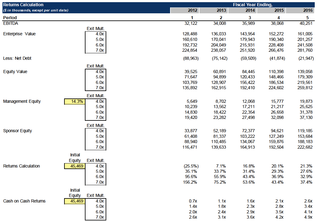
- The last portion of the model to complete is the Equity Returns schedule. This is essentially a simple calculation based upon the outputs generated by rest of the model.
- For each year, we simply take EBITDA multiplied by a range of purchase multiples to get to a total Exit Value for the company (Transaction Enterprise Value, or TEV).
- Next, we subtract out Net Debt (which is dependent on the 3-statement model you just created) to get to Equity Value.
- Next, we calculate the portion of the Equity Value that belongs to the management and the sponsor by using the initial equity breakdown for each party.
- From there it’s important to calculate both the internal rate of return (IRR) and the cash-on-cash returns (also known as the Multiple of Money or Multiple of Invested Capital). The only tricky part of this calculation is to make sure that you’re calculating IRR correctly, by using the correct Net Present Value or IRR formula and that, very importantly, you’re discounting by the right number of years! After all the mental energy you’ve expended to get to this point, it’s easy to make this mistake.
- Put simply, the IRR is equal to the cash-on-cash returns compounded by the number of years, minus 1. Thus, for example, for the 5-year, 5.0x Exit Multiple scenario:

- Put simply, the IRR is equal to the cash-on-cash returns compounded by the number of years, minus 1. Thus, for example, for the 5-year, 5.0x Exit Multiple scenario:
LBO Case Study: Conclusion and Final Comments
We hope that this case study provides some insight into all of the considerations that need to be made in building a realistic LBO model based on a case study in a Private Equity interview, and that the 9-step breakdown helps you simplify the task into easy-to-replicate and easy-to-execute steps.
No one becomes an expert LBO modeler overnight, so the key to doing well in this portion of the process is practice, practice, and more practice. With enough sample LBO cases, you should be able to master the steps needed to confidently build a fully functioning, professional LBO model on interview day.
Good luck with the modeling case and with the interviews!
←Paper LBO Model Example